Voiding the warranty: how the Kalman filter updates on data
There are a lot of excellent in-depth tutorials, derivations, and explanations of the Kalman filter that have already been written. The internet probably doesn’t need yet one more, and I can’t hope to fill such large shoes with one newsletter article.
But, with the Kalman filter occupying the direct intersection between probability and controls, I can’t think of better subject matter for These Are Systems.
So what I’m going to do is introduce the idea, talk briefly about how and why it works, and discuss what its limitations are (and aren’t). For those who haven’t heard of Kalman filters, perhaps it will pique your interest enough to look into them more deeply when an application arises.
The Kalman filter has two parts to it: predicting a system’s future state, and updating from measured data. In this article, I’ll focus on just the updating step, which is all you need for systems that don’t vary with time.
And for those who already know all about Kalman filters, you might still be surprised later on to see how far we can push them: in fact, this article is really about how you can take an approach that by all means shouldn't work and tinker with it a little bit until it does.
The power of brute force
In the previous post, I demonstrated a very general and accurate (but brute-force) technique for solving the lighthouse problem (locating a lighthouse at sea by random sightings of its light from the shoreline).
This technique works. In fact, as it adheres strictly to the axioms of probability theory and discards no information, I’m not sure it’s even theoretically possible for any other approach to do better, no matter how much cleverness was behind it.
But it’s also very computationally expensive. For the above two-parameter simulation, I had to evaluate the probability calculation on a grid of 20100 points, 1,000 times. Amazingly, we live in an era where that’s easily doable in a fraction of a second on a laptop computer — but as the problem dimensionality grows, this method gets hard, fast. If we were trying to estimate 10 parameters with a comparable grid density, we’d have ~100,000,000,000,000,000,000 probabilities to update at each step. That calculation quickly goes from taking half a second to taking a hundred million years.
I’m not saying it can’t be done, but sometimes we want to work smarter, not harder. And the Kalman filter is a pretty smart way to work.
If the Gaussian fits, wear it
First, we’re going to have to do something about this grid. Explicitly evaluating the probability of every plausible hypothesis across every new data point is just not going to be computationally scalable. But any alternative is necessarily going to discard something. What can we do?
A good approximation is like a good spam filter. It keeps everything you need, eliminates all the distractions you don’t care about, and generally gets out of your way when you’re trying to get your work done.
Remembering our Jaynes, approximation by a Gaussian is justified much more often than it might seem. So let’s see how far that gets us.
Instead of keeping track of the probability of every plausible value of a parameter, we’ll approximate our state of knowledge by a Gaussian distribution, keeping track of just the mean and variance. Instead of needing to evaluate hundreds of points for each parameter, we just have a few numbers to keep track of.1 That does mean we’re deliberately discarding some information, but in most cases, we’re retaining what is most important.
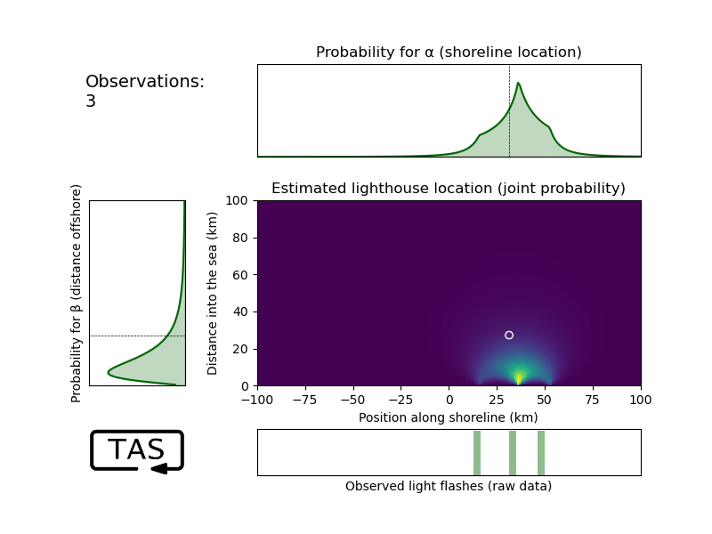
Let’s take a closer look at this lighthouse problem. When we had only a few data points, the distribution can get pretty exotic-looking:
With more data though, our probability estimate for the parameters does start getting very hard to distinguish from a Gaussian (even though the data is not Gaussian). It’s not perfect, sure, but it’s already a beautiful fit:
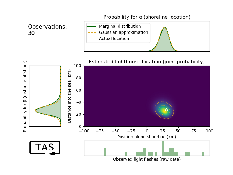
That goodness-of-fit is not a coincidence. It simply means that the first two moments of the probability distribution captures most of the relevant information, and it does little harm to discard the rest.
As you can see, in two dimensions, the Gaussian distribution has cross-sections in the shape of an ellipse.2 While the coloured area plot represents the most complete description of our state of knowledge, we could very accurately summarize it by a much briefer statement: the parameters of that Gaussian ellipse. That’s just five numbers: the center coordinates, minor and major axis lengths, and the tilt.
And five numbers is already a much more concise description than 20100.
Mathematically, a multi-parameter Gaussian is described by the following equation:3
The fraction at the beginning is just a normalizing factor to ensure the total area is 1; the interesting part that gives it its Gaussian shape is inside the exponent.
Here, y is the vector of unknown parameters, eg. [α, β]ᵀ
m is the total number of parameters in y, in this case 2;
μᵧ,ₖ is the vector of the means of our estimates for those unknown parameters y, as of the kᵗʰ data point; this locates the centre of the ellipse.
Sᵧ,ₖ is called the covariance matrix for y and describes how precisely we know α, β, and their joint combination (α + β) as of the kᵗʰ observed data point. You can think of it as the multidimensional version of the variance; it sets the axes of the ellipse:
Although Sᵧ,ₖ is an m × m matrix, it’s symmetric, so there are only 3 unique values in it. They represent the width of the ellipse in α and β, and its tilt.
(Actually, I apologize for the digression but I can’t resist the opportunity to do just a little bit better. This really deserves its own article, but it also belongs here.)
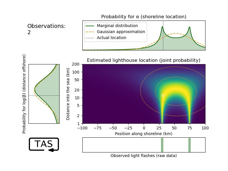
Both α and β are fit pretty well by a Gaussian, but you might have noticed that the fit for β isn’t quite as good; the marginal distribution (the plot on the left side) has a skew to it that the Gaussian can’t capture. And it also might be bothering you that, based on the premise of the lighthouse problem β can’t be less than zero, and yet the Gaussian distribution for β assigns a non-zero probability to negative values.
If these are indeed bothering you, then let me congratulate you on your sharp intuition. These are both clues that you get a much better fit by a change of variables from β → log(β).4 The fit to log(β) quickly converges rapidly and almost perfectly to a Gaussian, meaning that β’s distribution is better described as lognormal. This rather satisfyingly reflects β’s nature as a scale parameter.5 It means rewriting the Cauchy distribution like so:
So let’s try it. After only two observations, it’s already hard to distinguish the marginal probability distribution of log(β) from a Gaussian (even though α, and the joint distribution (α β), don’t look Gaussian at all yet):
But that’s just fine; there’s a 1-to-1 mapping between β and log(β), so it doesn’t cost us any extra to fit it to a Gaussian on log(β) rather than β. That’s what we’ll do going forward.
By the way, take a moment to appreciate how the joint distribution extracts a very clear story from those two points of data: “Either the lighthouse is close to shore and one flash was an outlier, or else it’s far from shore, in which case such spread-out data is to be expected.” This creates a Π-shaped curve of high likelihood, which the true location indeed happens to lie on. No Gaussian would ever be able to capture such nuance, which again goes to show that when data is scarce it’s worth making every ounce of effort in the analysis. When data is abundant, we can afford to play a bit more loosely.
The Kalman update procedure
OK. But calculating the exact joint probability distribution every time and then curve-fitting the result to a Gaussian is not going to save us any work at all.6 So now that we’ve compressed our probability distribution down to a Gaussian, how can we maintain this approximation as we update on new data?
Let’s look at what Bayes’ rule says:
Let me say that again in plain English:
So to update on the new data point xₖ₊₁, we essentially are multiplying our original distribution by the likelihood of that new data point.
In order for our approximation to work, we want to start with a Gaussian prior and end with a Gaussian posterior. As we update on the new observation xₖ₊₁, our goal will be to figure out how the mean (μᵧ,ₖ) and covariance (Sᵧ,ₖ) should be updated to get μᵧ,ₖ₊₁ and Sᵧ,ₖ₊₁.
Multiplying two functions together means adding their logarithms (that is, aᶜ×aᵈ = aᶜ⁺ᵈ). And the exponent of a Gaussian is a quadratic function — a parabola. That means we’re starting with a parabola, adding something to it, and we want the result to still be a parabola. That only works out exactly if the log-likelihood of xₖ₊₁ is either linear or a parabola itself; that is, if the data errors are exponentially or Gaussian-distributed.7
If that’s the case then after updating, the updated mean will located where the new parabola peaks, with the updated variance being its curvature. For a Gaussian, these are the only quantities we care about, so once we find them we’re done. And since parabolas are computationally inexpensive, the update equations are too.
This is what gives us the Kalman update equations, which for simplicity’s sake I’ll present here for the case of a single directly-measured parameter:8
The updated mean μₖ₊₁ will take what we’d expect based on the old estimate μₖ and move it a little bit, in proportion to how far away xₖ₊₁ was from where we expected it to be (μₖ);
The amount we move is also proportional to how uncertain we were in our old estimate σₖ², and how confident we are in our measurement. This is captured by the Kalman gain, Kₖ;
Our new uncertainty is correspondingly reduced by the same factor, as incorporating the additional data should make us more confident of our estimate.
In terms of code, this boils down to such a simple, fast procedure that it can run on an Arduino, a digital watch, or even the Apollo guidance computer.
And that is exactly how the Kalman filter updates on data.
Optimality
Rudolf Kálmán derived his filter assuming linear systems and Gaussian noise. When that assumption holds, it is the best possible linear filter.9 When the noise is furthermore uncorrelated in time (that is, the errors are independent), the Kalman filter is in fact optimal. Using just a few lines of linear algebra, it aligns exactly with what Bayes’ theorem suggests is the best possible analysis procedure. Nothing else we could do with the data, whether using machine or human brain, would yield a more reliable conclusion.
That’s a very powerful statement. If nothing else incites you to learn more about the Kalman filter, I hope that at least does.
Now, optimality is a great thing. But we started this discussion off by looking for approximations, and giving up perfection for efficiency’s sake. So what if we’re dealing with a problem where those assumptions don’t hold? Can the Kalman filter still serve us as a good approximation if, say, the noise isn’t Gaussian?
I have a feeling that more often than not, the map between problem and solution tends to be continuous: if problem B is near to problem A in some abstract “problem space”, then the solution for B usually won’t be too far from the solution for A in “solution space”.10
So even if its assumptions aren’t fully met, and even if its performance isn’t perfectly optimal, perhaps that doesn’t mean we need to throw away a useful tool.
Voiding the warranty
I chose to introduce the lighthouse problem for a reason: it’s very, very far from Gaussian.
The Gaussian distribution is a decent first-order approximation for any other distribution with the same mean and variance. But in the previous article, we observed that the lighthouse data follows a Cauchy distribution,11 and a Cauchy distribution doesn’t even have a mean or a variance. It has such long tails that its moments blow up if you dare try to calculate them. It’s so bad that taking the mean of the observation data never converges to the shoreline location α, not even close.
As far as error distributions go, the Cauchy might just be as non-Gaussian as it gets. It gets called “pathological” for a reason.
So if there is any application where you should be skeptical of applying a Kalman filter, this would be it. It’s the kind of proposal that could get someone laughed out of a meeting.
But do we have to let that stop us?
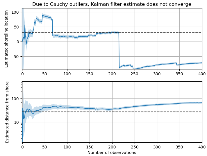
In a certain sense, yes. The Kalman filter, copied directly from a textbook, will choke as soon as it encounters a couple outliers.12
But maybe with an extra line of code, we can just ignore those outliers? After all, a Cauchy distribution with its tails chopped off has a finite mean and variance, so we should be able to proceed with this policy:
If the data point xₖ₊₁ is more than about ~3 μᵦ away from μₐ, ignore it for the purposes of estimating α;13
Otherwise, send the data to the Kalman filter as though it were Gaussian. (Even though it’s not).
Yes, this will introduce some distortions from Bayesian perfection, and we won’t be squeezing out every possible bit of information from each data point. For example, our estimate will now depend on the order of the observed data: if the first few data points happen to be clustered far to the left, and then the next few data points cluster far enough to the right that they get discarded, our model would be in a different state than if those same data had come in a different order. But as more data comes in, it eventually should correct. Is it the best we can do? No, discarding data is never the best we can do. But it takes only a minute to implement, and when data is abundant and compute resources are limited, it’s pretty darn good.
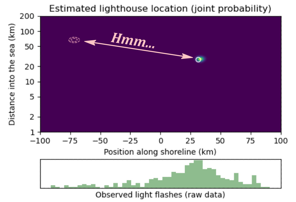
Ultimately, the proof is in the pudding, so here’s the pudding:
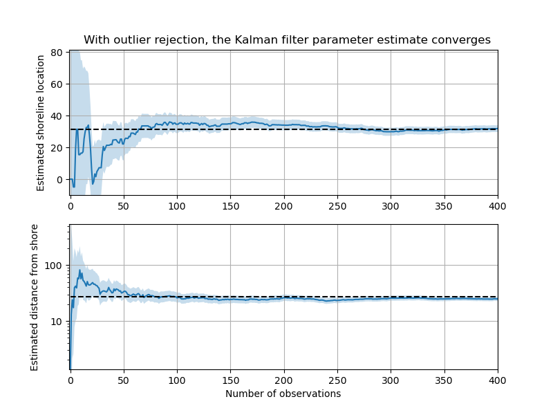
The pink dashed contours indicate the Kalman filter output, while the full Bayesian solution is shown for comparison in the coloured plot. It tracks well even though the Gaussian approximation is being computed without any reference to the brute-force probability distribution. Here is what the filter estimates look like over time, converging to the true value:
The Kalman filter is a powerful tool, and under some conditions unsurpassable. But even when the challenge at hand doesn’t meet those conditions, it’s still worth a try. Reasoning under uncertainty all comes down to making do with what you have, and a tool doesn’t need to reach perfection to still do exceedingly well.
And when we want to do better, we don’t have to throw the baby out with the bathwater. Small, intuitive improvements — a dash of change-of-variables, a pinch of outlier rejection — may be all it takes to challenge our preconceived limits.
Don’t get me wrong: it’s essential to have awareness of, and respect for, the assumptions and limitations of the tools that you use. But those assumptions are a lot like a sticker that says “warranty void if removed”. You can still remove it; you’re just relying on your own judgement if you do.
In fact, when I started writing this article, I didn’t even know whether I could make the Kalman filter work for this problem. But I trusted in Jaynes and thought it felt doable.14
This post isn’t intended as professional engineering advice. If you are looking for professional engineering advice, please contact me with your requirements.
We’ll be keeping track of the mean of each unknown parameter, its variance, and the covariance it shares with every other unknown parameter. For a system of n unknown parameters, that adds up to ½ n (n+3) values, which is a lot less than 100ⁿ values.
In fact, in any number of higher dimensions, the level curves of the Gaussian (that is, surfaces of equal probability) form an ellipsoid. Specifying the parameters of this ellipsoid is enough to uniquely specify the probability distribution.
If you aren’t familiar with the conventions of linear algebra, don’t be deterred. This is just a compact way of expressing the usual Gaussian form (y - μ)²/σ², but rearranged to look more like (y - μ)(1/σ²)(y - μ), and where y, μ, and σ are made up of various components. Expressing it in matrix form nicely captures how those components interact, without needing to fill the page full of terms like (α - μₐ)², (β - μᵦ)², and (α - μₐ)(β - μᵦ).
The way I think of it, when a change of variables like β → log(β) greatly simplifies a problem and makes the pieces fit, that’s not just some mathematical trick. It’s a sign of being one step closer to speaking the native language of the problem, or as Plato would say, “carving nature at its joints”.
There’s another big clue that thinking in terms of log(β) is the right way to think about this: even though the mean and variance of the Cauchy distribution cannot be calculated, remarkably the expectation of the measurement error ratio does exist, and I was happy to find it turns out to be exactly equal to log(β):
Better still, the integral for the variance of the above is also solvable, and is equal to π²/4.
You might remember from the previous article that ignorance of a scale parameter means we start with a uniform distribution over its logarithm, which is called the Jeffreys prior. If a state of total ignorance of β means a probability that is uniform over its logarithm, then it seems appropriate that more detailed knowledge of β gives us a Gaussian over its logarithm.
This is, however, sort of the spirit of the unscented Kalman filter, although it’s efficient about how it does so. There’s a good explanation here.
I haven’t yet seen a Kalman-filter-equivalent derived for exponentially-distributed errors, but from this observation it should be not only workable but exact, simple, and computationally efficient (although I’m not sure how it would handle the exponential’s lack of support below 0).
The Kalman filter actually permits a lot of flexibility in sensor arrangements. There can be multiple state variables being estimated at once, multiple sensors estimating each state variable (with different sorts of errors), and a state variable can also be unmeasured or indirectly measured, which means that you have to do a transformation of the measurements to determine how it relates to that state variable. I am not aiming to cover the general case in the scope of this article, as this isn’t an implementation guide. But the key tool that the Kalman filter uses is called the observation matrix, H, which projects the state vector onto the measurement vector.
When the state variables are directly measured (eg. state variable is temperature, measured by a temperature sensor), H is an identity matrix, and so it mostly disappears from the analysis.
There are extensions for the Kalman filter, such as the Extended Kalman Filter and the Unscented Kalman Filter, that help it deal with nonlinear systems, but that’s different than being able to handle non-Gaussian errors.
This is really the driving philosophy behind approximation in the first place. But to be sure, there are counterexamples.
The data is generated by a process that creates a Cauchy distribution. So if we knew precisely what the parameters α and β were, our best prediction for the next data point would also be a Cauchy distribution.
But we don’t even know α and β precisely: we know them only up to some mean and variance. This means that we should be even less confident in our prediction for x.
The distribution that reflects our uncertainty is really the convolution of a Cauchy over x with a Gaussian over its parameters. I’m not sure this distribution has any name, nor a nice closed-form expression. The closest thing might be the Voigt distrbution, which is obtained from a Cauchy with Gaussian uncertainty over the location parameter, but here we are uncertain of the scale parameter too. But anyway, we don’t really need to know the full distribution, just its mean and variance.
What it looks like if we don’t look before we leap: the occasional outliers overpower all the small, correct updates.
This is, by the way, a good example of why it’s worth learning and understanding the fundamentals, even for “solved problems” like Kalman filters. You can’t always rely on importing somebody else’s black-box code to solve your specific use case.
I don’t want this magic number “~3” to distract too much from the main idea, but you might wonder where it comes from. Basically, the variance of a cropped Cauchy distribution, with location parameter α and scale parameter β, that’s been bounded between (α-cβ, α+cβ) can be calculated as:
For the choice of bounds c = 2.798, this simplifies nicely such that the variance σ² = β². This corresponds to rejecting as outliers any samples where the lighthouse flash angle is suspected of being beyond ~70 degrees from the vertical, or about 22% of the data.
By the way, you might notice that this outlier-rejection procedure involves a kind of pulling ourselves up by our own bootstraps. When programming the filter, we don’t know the true values of α or β, so how do we know which points are truly outliers? We don’t; we can only discard data based on our parameter estimates. But if we have faith that the filter converges on an accurate estimate for β, we can trust that it will eventually be discarding the outliers correctly, which means that it should converge accurately on α, and so on.
This solution wasn’t pulled from a textbook, and while there is some literature on Kalman filters with non-Gaussian noise, I haven’t seen this very simple solution for Cauchy noise presented before. I don’t know if it is novel, although I’d be surprised if it were.

